Next: About this document ...
Up: Notes on the interactive
Previous: Notes on the interactive
Subsections
To generate tables of Rosseland mean (RM) opacities the user should specify a few
input parameters,
namely: 1) the
grid of the state variables, and 2) the
chemical mixture.
Please refer to the original paper by
Marigo & Aringer (2009, A&A, 508, 1539)
for all the details.
Below one finds practical indications on how to proceed.
For a given chemical mixture, one RM opacity table is
arranged as a rectangular matrix of dimension
 ,
where
,
where
 is the number of nodes of

 is the number of nodes of
![$ \log_{10}(R)=\log_{10}(\rho/[{\rm gr cm}^{-3}])-3\log_{10}(T) + 18$](img9.png) .
.
The lower and upper limits of
and
 and their grid spacing should be defined.
The default values are given in Table 1.1.
and their grid spacing should be defined.
The default values are given in Table 1.1.
| parameter |
min value |
max value |
grid spacing (dex) |

|
 3.2
3.2 |
 4.5
4.5 |
 0.01
for
0.01
for
|
| |
|
|
 0.05 for
|

|
 -8.0
-8.0 |
 1.0
1.0 |
 0.50 for
|
The user can specify different limits of the state variables,
provided that
 and
and
 ;
;
 and
and
 .
Also the grid spacing
.
Also the grid spacing
 ,
,
 ,
,
 can be
freely defined.
can be
freely defined.
It is specified by the user in terms of the following quantities:
It can be chosen among various options, listed in Table 1. Click on the bibliograpghic reference to view
the corresponding compilation of the individual metal abundances and the total metallicity, both in mass fractions and in number fractions.
Table 1:
Compilations of the solar chemical composition
|
|
 corresponds to the total abundance (in mass fraction) of metals, i.e. elements with
atomic number
corresponds to the total abundance (in mass fraction) of metals, i.e. elements with
atomic number  , of the reference mixture (see Sect. 2.5).
It can be freely chosen as a non-negative quantity,
, of the reference mixture (see Sect. 2.5).
It can be freely chosen as a non-negative quantity,
 .
.
It is expressed in mass fraction,
 , and can be freely chosen in the interval
 .
The user can define a sequence of increasing
.
The user can define a sequence of increasing  values, starting from
 up to
up to
 ,
with a step
,
with a step
 . This corresponds to compute a set of
![$ \color{blue} N_X={\rm int}[(X_{\rm max}-X_{\rm min})/\Delta X] + 1$](img42.png) opacity tables. To calculate one table, just set
opacity tables. To calculate one table, just set
 .
The elemental abundances can be expressed either in mass fractions,
.
The elemental abundances can be expressed either in mass fractions,  ,
or in number fractions,
,
or in number fractions,
 , according to:
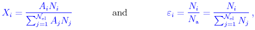 |
(1) |
where
 the number of elements,
  is the number density of nuclei of type
  with atomic mass
  , and
, and  is the
total number density of all atomic species (hydrogen, helium and metals).
In both cases the
normalization condition must hold, i.e.
is the
total number density of all atomic species (hydrogen, helium and metals).
In both cases the
normalization condition must hold, i.e.
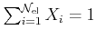 and
and
 .
.
The user should choose the preferred formalism,
and express the abundance variation factors of metals consistently
(see Sects 2.5 and 2.6).
For instance, if one wants to double the abundance of carbon with respects to its reference value,
it is necessary that ÆSOPUS knows whether the user's adopted abundance is in mass fraction, i.e.
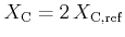 or in number fraction,
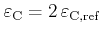 .
.
For those ones interested in metal-free mixtures (with
 ), having a
primordial
chemical composition produced by the Big-Bang nucleosynthesis, it is possible to specify the
abundance
of lithium, expressed by the ratio Li/H.
), having a
primordial
chemical composition produced by the Big-Bang nucleosynthesis, it is possible to specify the
abundance
of lithium, expressed by the ratio Li/H.
The
default configuration assumes
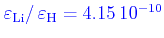 as predicted by the standard Big-Bang nucleosynthesis in accordance with the
WMAP results (Coc et al. 2004).
as predicted by the standard Big-Bang nucleosynthesis in accordance with the
WMAP results (Coc et al. 2004).
2.6
Reference mixture
Please refer to Sects. 3.1 and 4.3 in
Marigo & Aringer (2009, A&A submitted)
for more details and applications to
 -enhanced mixtures.
By construction the reference mixture has a metallicity
 , previously selected by the user.
The reference abundances of the metals,
 or
or
 are defined by the ratios (in dex):
![$\displaystyle \color{blue}[A_i/{\rm Fe}] = \log \left(\frac{X_{i, {\rm ref}}}{X_{\rm Fe, ref}}\right) -\log \left(\frac{X_{i,\odot}}{X_{\rm Fe,\odot}}\right)$](img62.png) |
(2) |
or
![$\displaystyle \color{blue}[A_i/{\rm Fe}] = \log \left(\frac{\varepsilon_{i, {\r...
...t) - \log \left(\frac{\varepsilon_{i,\odot}}{\varepsilon_{\rm Fe,\odot}}\right)$](img63.png) |
(3) |
which should be specified in the interactive mask. For each selected species the ratio can be set either
positive
(corresponding to
supersolar ratios), or
negative (corresponding to
subsolar ratios).
The
default configuration assumes
![$ \color{orange}[A_i/{\rm Fe}]=0$](img64.png) for all metals, i.e. the reference mixture
consists of
scaled-solar abundances.
for all metals, i.e. the reference mixture
consists of
scaled-solar abundances.
Once specified the
![\bgroup\color{orange}$ \color{orange}[A_i/{\rm Fe}]$\egroup](img65.png) ratios for the
selected elements, the user should decide
how the reference mixture is constructed in order to preserve the reference metallicity, namely:
ratios for the
selected elements, the user should decide
how the reference mixture is constructed in order to preserve the reference metallicity, namely:
-
Mixture
 The total abundance variation of the
selected metals is balanced by the
abundance variation of
all other metals.
The total abundance variation of the
selected metals is balanced by the
abundance variation of
all other metals.
-
Mixture
 The total abundance variation of the
selected metals is balanced by the
abundance variation of
iron-group elements.
The total abundance variation of the
selected metals is balanced by the
abundance variation of
iron-group elements.
Frequent applications of this setting section likely deal with
 -enhanced mixtures, i.e. with supersolar ratios
![\bgroup\color{orange}$ [\alpha/{\rm Fe}]$\egroup](img69.png) of
-elements (O, Ne, Mg, Si, S, Ca, and Ti).
of
-elements (O, Ne, Mg, Si, S, Ca, and Ti).
2.7
Additional chemical pattern
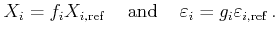
Finally, superimposed to the reference chemical mixture it is also possible to specify an additional chemical pattern,
defined by the
abundance enhancement/depression factor
 or
or
 of each metal species (heavier than helium),
with respect to its reference abundance.
of each metal species (heavier than helium),
with respect to its reference abundance.
 |
(4) |
In the web-mask the user should specify the decimal logarithm of the variation factors:
 or
or

The
default configuration assumes
 or
or
 for all metals, i.e. the final mixture coincides with the reference mixture.
Where the variations factors of the
selected elements are set
 (or
(or
 ), then the actual metallicity
 ,
i.e. the enhancement/depression factors
,
i.e. the enhancement/depression factors
 of the selected elements
produce a net increase/depletion of total metal content
of the selected elements
produce a net increase/depletion of total metal content
 relative to the reference metallicity
 .
.
In this case all
 variation factors
can be freely specified without any additional constrain.
variation factors
can be freely specified without any additional constrain.
These optional settings should be of particular interest to researchers dealing with
the
atmospheres of TP-AGB stars, as their C/O ratio,
as well as the absolute C, N, and O abundances, may be significantly altered by the occurrence
of the third dregdge-up and hot-bottom burning.
For the three composition parameters, the user can define a few values (in dex),
each sequence corresponding to a grid of opacity tables.
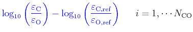
For instance, let us suppose that the selected normalization of the abundances is in number fraction, then
one can choose the variation factors defined as:
Note that, by construction, the variation factors for O are given by
 .
.
Filling in these fields will supersede
the variations factors for C, N, and O set in the previous mask
(see Sect. 2.6).
The maximum allowed numbers of values are:
 ;
;
 ;
;

ÆSOPUS computes RM opacity tables for
all combinations of
 ,
,
 , and
, and
 .
.
It follows that the
total number of tables (for given
)
is
 .
.
Pay attention that the resulting number of tables may become quite high!
Next: About this document ...
Up: Notes on the interactive
Previous: Notes on the interactive
Paola Marigo
2009-06-26